The niftiness and diversity of consistent hashing

I’ve been interested in decentralized data in distributed systems lately. There’s too much data for any one storage node to handle, so you have lots of storage nodes and each gets some of the data. But how do you decide which node is responsible for a certain data item?

The problem space is diverse. In peer-to-peer systems, nodes just sort of have data that they register with the network. They have to not only find the node that has data, but also find out what data exists in the first place. Then there are distributed key/value systems like the one described in Amazon’s Dynamo paper. Data is placed in storage to balance the load and replicated across nodes to increase resiliency. And then there are CDNs and cache systems. In decentralized caches like the one described in the original consistent hashing paper, clients make an educated guess about the cache node that holds the data they’re looking for, and the design goal is to give each client a way to guess right most of the time with limited information.

I think the last problem is interesting: How can we make an educated guess about what storage node might have the data when we only have partial information about the network? It requires a bit of an intuitive leap.

Each data item is represented by a key, so there’s some concept of a key space, which represents all possible data keys. We can use a hash space as a pretty effective proxy for the key space, and then partition that hash space into ranges. Each storage node in our system becomes responsible for one of the ranges in the hash space.¹

A hash space is the set of possible outputs of a hash function – for example a SHA1 hash is 160 bits, so the hash space is all integers from 0 to 2¹⁶⁰. We know that if we hash different keys, we’re very likely to get different hash values, so this satisfies the “hash space as proxy for all possible keys” criterion. And hash functions are reasonably unbiased, so a hashed key has essentially equal probability of landing anywhere between 0 and 2^n_bits. The hash space is essentially a number line, and we can make it continuous by connecting the tail back to the head, so that the successor of the largest hash value is the smallest hash value.

You place a data item on the ring by hashing its key.

pos_x = sha1(x.key)

Our storage nodes are each responsible for a range, so we need a way to define these ranges. To that end, we place nodes on the ring as well, by hashing their IP addresses.

pos_server = sha1(s.ipaddr)

We decide that each node is responsible for the hash values between itself and its predecessor, which is to say the range of hash values between itself and the nearest counter-clockwise neighbor on the hash ring.

With a 64-bit hash space and 10 nodes, you might end up with a configuration like this.

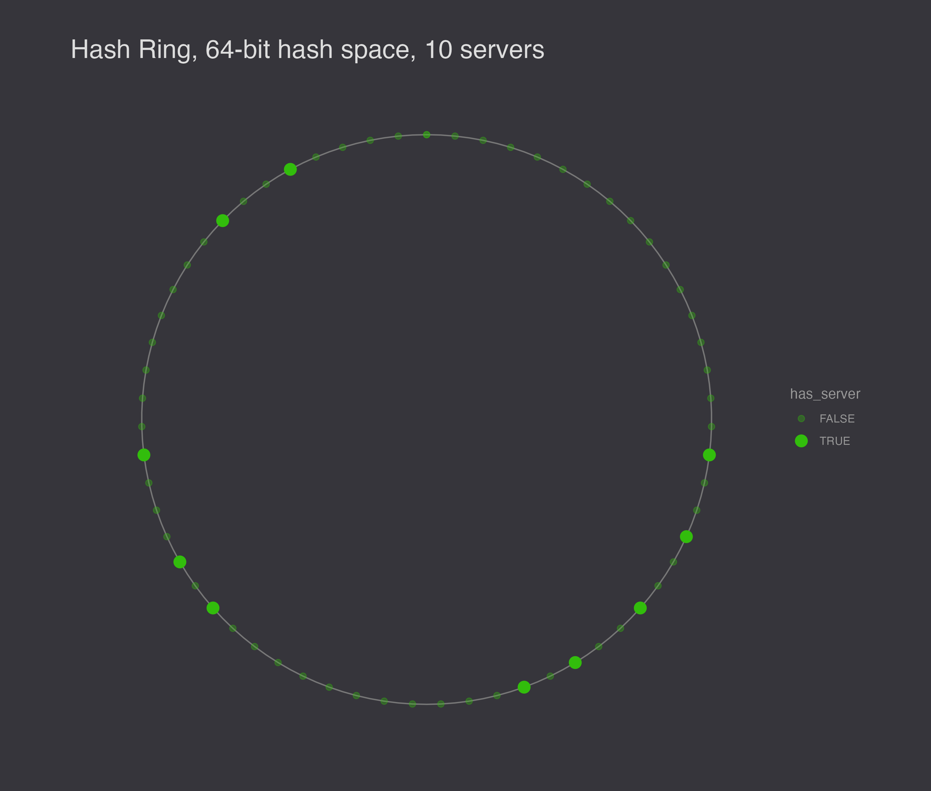
Now if a client knows about any set of storage nodes, it can make its own partition of the hash ring and be mostly correct! If the client knows about 9 out of 10 nodes, when it makes its partition of the hash ring, it will correctly identify 8 out of the 10 actual ranges, and it won’t do too badly guessing about the 9th and 10th ranges, either.

Here’s how consistent hashing scores on a few more criteria:

• Precise. About as accurate as you can be with limited information about storage nodes.
• Deterministic. Yep.
• Equal distribution of work. The hash ring is reasonably well distributed, but it’s not perfect. The size of each range is random.
• Adaptable to changes in membership. This is one of the main motivations for consistent hashing. If you add a node, it divides some existing range, and the only redistribution that happens is with the new node’s successor. If you remove a node, the successor node becomes responsible for the range of the node that left, but no other nodes are affected.

In cache systems, getting close to the right node is good enough. Even if a node isn’t technically responsible for a key, it can still request the key from the server and cache the key itself. Any other clients that have the same incomplete information about the network will hit this (non-responsible) node and find the cached data there. Responsibility in this system is weak, but the data is stored with a lot of locality relative to the hash ring.

Sometimes you need to find exactly the node responsible for a key. The Chord protocol provides such stricter routing. When a server joins the network, it notifies its neighbors and then learns about them. The protocol ensures that the new node knows a lot about its immediate location on the ring, but less about the nodes that are farther away from it. When a client makes a data request to find a key, it reaches out to any node on the network. This node probably doesn’t have the data, but it knows someone who is close. The storage node forwards the request counter-clockwise (backwards) on the ring to the closest node to the point where the key is, but without passing it. This node could be the owner of the data item, but if it’s not, it knows enough about its local area on the ring to find a node that’s closer to to it. The routing tables are built in such a way that if a node doesn’t know of any closer node to the data item, it is the owner of the data item.²

The number of hops in a Chord data retrieval is bounded. Latency isn’t optimal, because there may be some number of hops to find the data, and in fact the nearness on the ring says nothing about how close two nodes are in the world. This is one of the hard problems of overlay networks, but there are optimizations for it.

So, different systems treat the routing requirement differently. A cache system is able to relax the routing requirement, because it tries to reduce cache misses but not prevent them entirely. Chord meanwhile guarantees that a key is found. It’s a scalable protocol that works in very unstable networks, at the cost of extra latency.

There are still a few issues. First, a node leaving is likely to increase the workload for another node, and a node entering the ring is likely to divide another node’s workload while leaving the remaining nodes with the same workload. Second, random positions on the ring are not very likely to be evenly spaced. (There is after all only one evenly spaced configuration.) Third, the scheme ignores heterogeneity – some servers can handle more work than others.

To illustrate the load balancing problem with hashing servers to the hash ring, I generated 10 different random configurations to show that they are not generally evenly spaced.

Next, I simulated 1,000 requests for data, and I ran the simulation 10 times, plotting the results. In this plot, the size of the node represents the number of requests serviced at the node.

If we want to smooth out the load, the solution is to assign each server a number of random virtual nodes on the ring. Virtual nodes decrease the chances that a node gets a particularly big range of responsibility on the ring – instead of getting unlucky once, it would have to get unlucky N times in a row for N virtual nodes per storage node.

Here’s another 1,000 requests made to a ring with 32 nodes instead of 10. I ran the simulation 10 times and plotted each outcome.

If you take any N nodes (say 4) and average their size, you get a reasonable number of requests. We can also solve the heterogeneity problem by allocating servers a number of virtual nodes according to its abilities. Finally, membership changes more evenly rebalance the nodes. When a node is removed, its virtual nodes are removed from the circle, and the extra work is split among all of the owners of the virtual nodes’ successors. It’s very likely that the successors will be owned by several nodes, not just one.

Routing is a little more complicated. The system needs to store some amount of extra metadata about how to map virtual nodes to actual nodes. For this reason, virtual nodes are most effective in smaller systems where each storage node might be responsible for a large chunk of the hash ring.

The design space becomes expansive at this point as particular systems balance metadata and latency with other guarantees they need to make. But this is the essence of the thing. We create a proxy for the key space that tends to evenly distribute nodes and then divvy up that domain across the storage nodes. Elegant, if you ask me.

Sources

• Consistent Hashing and Random Trees: distributed caching protocols for relieving hot spots on the world wide web
• Chord: a scalable peer-to-peer lookup service for internet applications
• Dynamo: Amazon’s highly available key-value store
• Distributed Systems, 4e, by Maarten Van Steen and Andrew S. Tenenbaum (link)
• Computer networks: a systems approach, 3e, by Peterson and Davie

1. There are lots of ways to transform and then partition a key space, but most don’t work well. It’s vital that all keys are distributed evenly across storage nodes. So you might try to partition the key space by prefix and then place the key on the server whose name has the same prefix. This doesn’t work well because (a) there’s no guarantee that servers will have distinct prefixes, especially when they’re in the same subnet, (b) if they do have distinct prefixes, they’re probably not evenly spaced, and (c) you become significantly limited in the number of buckets. The longest prefix for an IPv4 address is 32 bits. ↩

2. See also Pastry, which optimizes the routing tables differently. ↩